Tuning a sensing dot

pieter.eendebak@tno.nl

In this notebook we show how to tune a sensing dot to a sensitive point. We assume the dot is controlled by 3 gates: a single plunger gate and two barrier gates.

First we load a station

%matplotlib inline
import os
import users.eendebakpt
startfile = os.path.join(os.path.split(users.eendebakpt.__file__)[0], 'start8dot.py')
exec(open(startfile, 'rt').read())

gv={'B0': 100.0, 'B1': -255.0, 'B2': -330.0, 'B3': 100.0, 'B4': 100.0, 'B5': 100.0, 'B6': 100.0, 'B7': 100.0, 'B8': 100.0, 'D0': -230.0, 'O1': 0.0, 'O3': 0.0, 'O5': 0.0, 'P1': 100.0, 'P2': -110.07858396276811, 'P3': -84.992751964598938, 'P4': 100.0, 'P5': 100.0, 'P6': 100.00762951094839, 'P7': 100.00762951094839, 'P8': 100.0, 'X1': 15.0, 'X2': 51.0, 'Y0': -250.0, 'Y1': -375.0, 'Y2': -405.0, 'Y3': -520.0, 'phase': 0.0}
gates.resetgates(gv,gv, verbose=0)

Windows foundInitialized IVVI-rack in 0.07s
Connected to: KEITHLEY INSTRUMENTS INC. 2000 (serial:4045453, firmware:B01  /A02) in 0.10s
Connected to: KEITHLEY INSTRUMENTS INC. 2000 (serial:1264625, firmware:A20  /A02) in 0.06s
Connected to: TEKTRONIX AWG5014 (serial:B010188, firmware:SCPI:99.0 FW:3.3.182.755) in 0.12s
Connected to: TEKTRONIX AWG5014 (serial:B010106, firmware:SCPI:99.0 FW:3.1.141.647) in 0.18s
Connected to: Rohde&Schwarz SMB100A (serial:1406.6000k02/106309, firmware:3.0.13.0-2.20.382.35) in 0.02s
connected to fridge: mc 53.6 [mK] at 14-03-18 10:42:11
initialized XLD8dot
started calibration master

The sensing dot is defined by the sensingdot_t structure. The main arguments are the gates to control the dot and the instrument used to read the current through the dot. The code also works for fast readout (e.g. with RF), but the RF readout should be tuned beforehand.

sd=qtt.structures.sensingdot_t(['Y0', 'X1', 'Y1'], station=station, index=1, minstrument=(station.digitizer, 1))
print(sd)

sd gates: Y0, X1, Y1

Basic checks

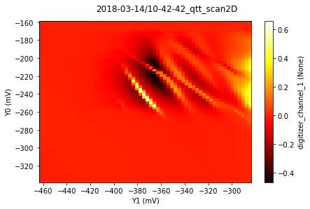
First we check that we have a dot defined by making a barrier-barrier scan. This scan only needs to be done once or when the system is not functioning properly.

ds=sd.scan2D(ds=90, fig=100, stepsize=4., verbose=0)
print(ds)

`sensing dot sd gates: Y0, X1, Y1: performing barrier-barrier scan
DataSet:
   location = '2018-03-14/10-42-42_qtt_scan2D'
   <Type>   | <array_id>          | <array.name>        | <array.shape>
   Measured | digitizer_channel_1 | digitizer_channel_1 | (60, 60)
   Setpoint | Y0                  | Y0                  | (60,)
   Setpoint | Y1                  | Y1                  | (60, 60)

Automatic plunger calibration

The most sensitive part of the sensing dot is the plunger calibration. We calibrate this by making a 1D plunger scan and analysing the Coulomb peaks. The sd.fasttune method uses an Arbritrary Waveform Generator to sweep the voltage applied on the plunger gate.

plungervalue, dataset = sd.fastTune(fig=200)

sensingdot_t: autotune complete: value 18.7 [mV]

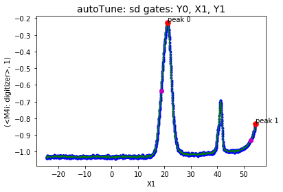
We have found a good Coulomb peak that can be used for sensing. The plungervalue is at the position of half-height on the left of the main peak is given by plungervalue. The detected peaks are stored in sd.goodpeaks.

print(sd.goodpeaks[0])

{'p': 1075, 'x': 21.290724119600114, 'y': -0.22793701171875, 'gaussfit': array([      144.056,        22.218, -74289121.491]), 'halfvaluelow': -0.63338573608398441, 'height': 0.81089744873046876, 'valid': 1, 'lowvalue': -1.0388344604492188, 'type': 'peak', 'phalf0': 1015, 'phalfl': None, 'indlocal': range(160, 1075), 'xhalfl': 18.747484760607783, 'xfoot': 16.83929856711743, 'yhalfl': -0.6355261230468756, 'pbottomlow': 959, 'pbottom': 980, 'pbottoml': 980, 'xbottom': 17.242719804605507, 'xbottoml': 17.242719804605507, 'vbottom': -0.92364990234375, 'ybottoml': -0.92364990234375, 'score': 1.1093033796349248, 'slope': 0.22611322194339117, 'heightscore': 0.89987918779906506, 'scorerelative': 1.4348433638937708, 'noisefactor': 0.9999280126696406}

Optimizing the sensing dot

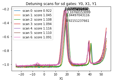
Optimizing the sensing dot is something that requires some experience and knowledge of the sample. It is also a balance between sensitivity (sharpness of the peak) and range (width and height of the peak). When performing single-shot read-out sensitivity is more important, while a relatively larger range is typically preferred for measuring a charge-stability diagram. However, a general rule of thumb is that the sensing dot peak is best when it is symmetric (e.g. the tunnel rates for the two tunnel barriers are equal). To determine the optimal detuning one can use the detuning_scan function.

optimal, results = sd.detuning_scan(nsteps=7, stepsize=3.5, fig=100)

detuning_scan: iteration 0: detuning -7.500
sensingdot_t: autotune complete: value 16.8 [mV]
detuning_scan: iteration 1: detuning -5.000
sensingdot_t: autotune complete: value 17.0 [mV]
detuning_scan: iteration 2: detuning -2.500
sensingdot_t: autotune complete: value 17.8 [mV]
detuning_scan: iteration 3: detuning 0.000
sensingdot_t: autotune complete: value 15.1 [mV]
detuning_scan: iteration 4: detuning 2.500
sensingdot_t: autotune complete: value 15.5 [mV]
detuning_scan: iteration 5: detuning 5.000
sensingdot_t: autotune complete: value 16.1 [mV]
detuning_scan: iteration 6: detuning 7.500
sensingdot_t: autotune complete: value 16.9 [mV]
detuning_scan: best 4: detuning 2.500

Calibration of RF readout

…